When batch effects dominate, biology disappears. Same samples, same coordinates — only the coloring changes.
Batch variance
PC1 explains 62% — almost entirely sequencing run, not biology.
TL;DR
Batch effects are technical variation introduced when samples are processed at different times, by different people, or on different machines.
They can completely mask the biological signal you are trying to find.
TransXplorer detects them automatically using PVCA + kBET + Silhouette and corrects them with limma's removeBatchEffect — one click.
Section 01
What batch effects actually are
A batch effect is technical noise in your data that looks like biology. More precisely, it is systematic variation between groups of samples that traces back to how the samples were processed, not what they actually are.
Imagine you sequenced ten control mice on Monday and ten treated mice on Friday. The reagent lot was different. The instrument had been recalibrated. A different technician loaded the flow cell. Now when you compare expression between treated and control, you cannot tell which differences came from your treatment and which came from running the samples four days apart. The two sources of variation are tangled together.
Batch effects are sneaky for one reason: they look statistically real. Genes will appear to be differentially expressed between groups with low p-values and respectable fold changes. The math is not lying. The samples really do differ. But the difference is technical, not biological — and that is precisely what makes batch effects dangerous. They mimic the signal you are looking for.
Common sources include:
Different sequencing runs or lanes on the same instrument.
Different reagent lots (library prep kits especially).
Different operators handling the samples.
Different processing dates, even by a few days.
Different sample storage conditions or freeze-thaw cycles.
Different centers in a multi-site study.
The first defense is always experimental design: randomize samples across batches so that each condition is represented in each batch. We will get back to this later. But even with the best design, batch effects almost always sneak in — which is why detection and correction matter.
Section 02
The famous case — when batch effects pretend to be biology
The cautionary tale every bioinformatics class tells is the one Leek and colleagues used to anchor their 2010 review in Nature Reviews Genetics. Reanalysing a high-profile expression study of population differences, they noticed that the apparent biological signal was almost perfectly aligned with the date each batch of arrays had been processed. The strongest "ancestry" axis in the data was, in fact, mostly time.
The original 2007 paper by Akey and colleagues had concluded that human populations differed in the expression of many genes. The reanalysis showed that many of those genes also differed between processing dates — and because population happened to be confounded with date, the two effects could not be told apart. Once batch was accounted for, a large fraction of the reported population differences shrank or disappeared.
The lesson is uncomfortable but important: if your biological variable is confounded with batch, no statistical method can fully save you. Correction tools can adjust for batch only when the data contain enough information to distinguish batch from biology — and a confounded design destroys that information by construction.
The takeaway
Good experimental design comes first. Randomize samples across batches. If you cannot — for example, because one cohort was collected years before the other — document it, be honest about it in the paper, and apply correction with care. Reviewers know to look for this.
That 2010 review (Leek et al., Nat Rev Genet 11:733–9) is still the single best read on why this matters. The takeaway from the Akey case is not "those authors were sloppy" — it is that batch effects are so easy to miss that they have caught even careful, well-funded labs by surprise. Assume they are present in your data until you have proven otherwise.
Section 03
How to detect batch effects
A quick visual sanity check is to run a principal component analysis (PCA) and color the samples by batch. If the points cluster by batch rather than by biology, you have a problem — like the hero plot at the top of this page. But the eye is unreliable, so the field has developed three complementary quantitative metrics. Each one asks a slightly different question, and using them together is more robust than picking a favourite.
PVCA — Principal Variance Component Analysis
PVCA decomposes the total variance in your dataset into named sources: batch, condition, the batch×condition interaction, and unexplained residual variance. The output is one number per source — the percentage of variance attributable to it.
Rule of thumb: if batch explains more than ~10% of variance, you have a meaningful batch effect. If it explains 30% or more, your biological signal is almost certainly drowning. Researchers also watch the batch×condition interaction term — a large interaction means batches behave differently across conditions, which complicates correction.
PVCA — variance decomposition
fig 3.1
Reading the bar: if the red bar (batch) is larger than the blue bar (condition), your batches differ more than your biological groups. That is a red flag — almost always literally.
kBET — k-nearest-neighbor Batch Effect Test
kBET takes a different angle. For each sample, it looks at its k nearest neighbours in expression space and asks: do those neighbours represent batches in roughly the same proportion as the dataset overall? If yes, batches are well-mixed locally and there is no batch effect. If neighbours are mostly the same batch, samples are segregating by batch.
The output is a rejection rate: the fraction of neighbourhoods that fail the mixing test. A value below ~0.1 indicates clean data; values approaching 1.0 mean samples cluster almost entirely by batch.
kBET — neighbourhood batch mixing
fig 3.2
Reading the circles: a kBET neighbourhood (dashed) should contain the same batch ratio as the full dataset. On the left, the circle holds blue, red, and green points equally — well mixed. On the right it contains only red — batch effect.
Silhouette score
The silhouette score measures how well each sample fits its assigned cluster compared with the nearest other cluster. When clusters are defined by batch label, a high silhouette means samples sit comfortably with their own batch and far from others — i.e. batches separate cleanly. A low or negative silhouette means batches are intermixed.
Counterintuitively, you want a low silhouette by batch. The interpretation is the opposite of normal silhouette use: if your batches form tight, well-separated clusters, that is bad news for downstream analysis.
Silhouette by batch — threshold gauge
fig 3.3
Reading the gauge: a silhouette < 0.25 means batches are well-mixed. Between 0.25 and 0.5, you have a moderate effect worth correcting. Above 0.5, your batches are forming clean clusters — correction is essential.
One score, no guesswork
TransXplorer runs all three metrics automatically and surfaces a unified score on the Quality Control tab. You do not need to pick a favourite or know which thresholds matter — the platform highlights anything concerning and tells you whether to correct.
Section 04
How to correct batch effects
Once you have confirmed a batch effect, the next question is which correction method to use. The right answer depends on what your data looks like and whether you know your batch labels. Three methods cover almost every practical case.
limma::removeBatchEffect
Recommended · used by TransXplorer
Linear-model adjustment for log-transformed expression data — the engine behind TransXplorer's one-click correction.
removeBatchEffect fits a linear model with batch (and any other nuisance factors) as covariates, then subtracts the estimated batch contribution from each gene. Critically, it accepts a design matrix describing the biological effects you want to keep, so the model can adjust for batch without erasing your condition. TransXplorer auto-applies the correct log transform (voom-style log2(counts+1)) before the call, so you do not need to think about input format.
Operates on log-transformed expression (voom output, log-CPM, or log2(counts+1)).
Linear-model framework integrates cleanly with the rest of the limma DE pipeline.
Preserves biology of interest via the design argument — what TransXplorer passes by default.
Ritchie ME, Phipson B, Wu D, Hu Y, Law CW, Shi W, Smyth GK (2015). limma powers differential expression analyses for RNA-sequencing and microarray studies. Nucleic Acids Research 43(7): e47. doi:10.1093/nar/gkv007
ComBat-seq
Empirical Bayes adjustment designed specifically for RNA-seq count data — a common alternative when you need to keep integer counts.
ComBat-seq is the modern successor to ComBat, redesigned to work directly on integer counts rather than log-transformed data. It models each gene as a negative binomial distribution per batch, estimates batch-specific location and scale parameters, then adjusts each count to what it would have looked like in a reference batch — while preserving the count distribution downstream methods like DESeq2 and edgeR depend on.
Operates on raw counts — preserves the integer count structure required by DESeq2/edgeR.
Empirical Bayes shrinks batch-effect estimates toward a global mean — more stable when batches contain few samples.
Accepts a covariate of interest (your biological condition) so it can adjust for batch without removing biology.
Zhang Y, Parmigiani G, Johnson WE (2020). ComBat-seq: batch effect adjustment for RNA-seq count data. NAR Genomics and Bioinformatics 2(3): lqaa078. doi:10.1093/nargab/lqaa078
ComBat
The original 2007 method — built for microarrays and log-transformed data.
ComBat is still in wide use, but it assumes the input is approximately normally distributed — which is true for log-CPM or log-TPM values but not for raw counts. Applying ComBat directly to integer counts distorts the variance structure and breaks downstream count-based methods. Reach for ComBat only when your data are already log-scale (microarray intensities, or RNA-seq that has been variance-stabilized).
Empirical Bayes shrinkage like ComBat-seq, but on the log/normal scale.
Good for microarray expression, methylation beta-values, or VST/RLOG-transformed RNA-seq.
Not appropriate for raw integer counts.
Johnson WE, Li C, Rabinovic A (2007). Adjusting batch effects in microarray expression data using empirical Bayes methods. Biostatistics 8(1): 118–127. doi:10.1093/biostatistics/kxj037
SVA / RUV
When you do not have batch labels — recover the unwanted variation from the data itself.
Sometimes you inherit a dataset and the metadata simply does not record which samples were processed together. SVA (Surrogate Variable Analysis) and RUV (Remove Unwanted Variation) infer hidden sources of variation by looking for systematic patterns that are not aligned with your biological variable. The recovered "surrogate variables" can then be included as covariates in your differential-expression model.
Useful when batch labels are missing or untrustworthy.
RUV often uses negative control genes (e.g. housekeeping genes) as a reference for what should not vary.
More conservative than ComBat-seq — it adds covariates to the model rather than rewriting your counts.
Leek JT, Storey JD (2007). Capturing heterogeneity in gene expression studies by surrogate variable analysis. PLoS Genetics 3(9): e161. · Risso D et al. (2014). Normalization of RNA-seq data using factor analysis of control genes or samples. Nature Biotechnology 32: 896–902. doi:10.1038/nbt.2931
Batch correction is not a magic eraser. If batch is confounded with your biological variable — meaning all treated samples were run in one batch and all controls in another — then any algorithm that removes batch differences will also remove biological differences. The two are mathematically indistinguishable. You will get clean PCA plots and no DEGs.
The fix is upstream of any software: balance your design so each batch contains samples from each condition. Even a small amount of mixing rescues correction. The diagram below contrasts a fatal confounded layout with a balanced one.
Confounded vs balanced experimental design
fig 5.1
Rule of thumb: if you cannot draw a line through the design grid such that each row and column contains samples from each condition, your design is at risk. Mix the conditions across batches before sequencing — not after.
When over-correction shows up
Symptom: after applying batch correction, you have fewer DEGs than before, the volcano plot empties out, and PCA shows all samples in one cloud regardless of condition. This means the correction stripped real biology along with batch. Go back, examine your design matrix, and make sure your biological condition is in the design argument of limma::removeBatchEffect (or supplied as a covariate to ComBat-seq) so the model knows to protect it.
Section 06
Decision flowchart — should I correct?
Here is the path most analyses follow. Read top-to-bottom: at every question, NO branches left and YES branches right. Red end-states mean stop and rethink; green means you are clear to proceed.
Should I correct for batch effects?
fig 6.1
Reading the chart: NO branches left, YES branches right. In TransXplorer, only the first two questions need a human answer — the platform applies the correct log transform, calls limma::removeBatchEffect with your biology preserved in the design matrix, and recomputes PVCA so you can confirm the fix.
Section 07
How TransXplorer handles all this
Everything above — PVCA, kBET, Silhouette, limma::removeBatchEffect, SVA fallback, the re-check after correction — is wired into the Quality Control tab. You upload your counts and metadata, and the platform takes care of the workflow:
Auto-detection on upload. The moment your data are in, TransXplorer computes PVCA, kBET, and Silhouette in parallel and surfaces a unified batch-effect score with a clear “clean / moderate / strong” verdict.
Visual report. A stacked variance bar (PVCA), a sample-neighbourhood mixing chart (kBET), and a silhouette gauge all in one panel, with the thresholds annotated — no guesswork.
One-click correction. When batch labels are present in your metadata, TransXplorer log-transforms your counts and calls limma::removeBatchEffect with a design matrix built from your biological condition, so batch is removed while the biology of interest is preserved. If batch labels are missing, the platform falls back to SVA-derived surrogate variables.
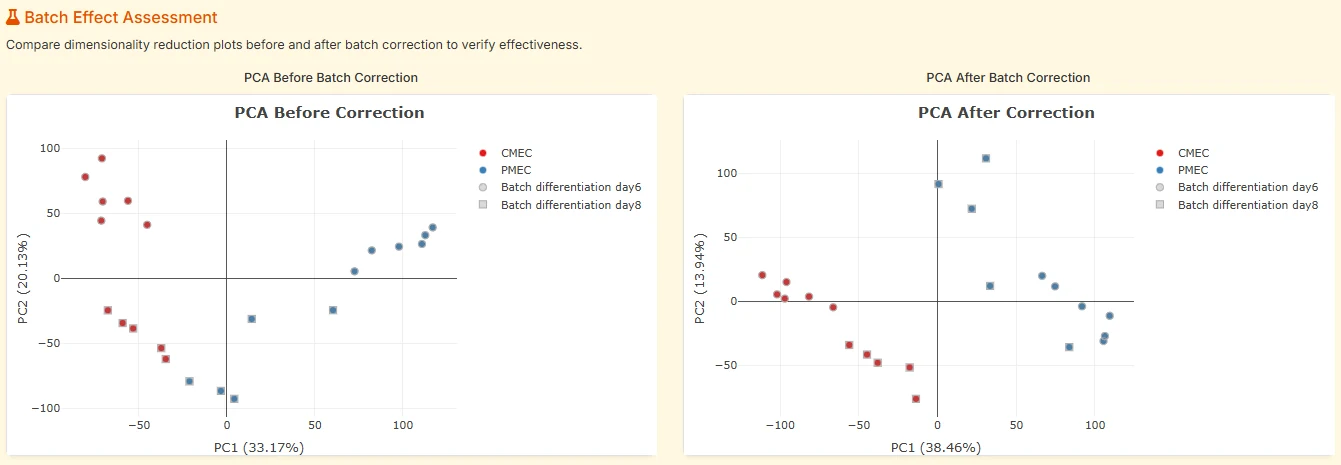
Before/after PCA. A side-by-side PCA plot lets you see, visually, whether batch separation collapsed after correction — like the hero illustration but on your own data.
Methods-ready text. TransXplorer auto-generates the Methods section sentence with the version numbers and parameters used, so it drops straight into your manuscript.
fig. 7Before/after PCA in TransXplorer's batch assessment panel. Left: samples cluster by sequencing batch (day6 vs day8) along PC2. Right: after limma::removeBatchEffect, samples cluster by biology (CMEC vs PMEC) and batch separation has collapsed.
The whole loop runs in your browser. No R, no Python, no Docker. If your data fits in a counts CSV, batch detection takes about ten seconds and correction another five.
Try batch detection on your own data
Free, browser-based, no login. Drop a counts file in and TransXplorer will tell you within seconds whether your data needs correction.
Five mistakes that turn up over and over in published RNA-seq analyses. Each one is avoidable.
Confounding batch with biology.
The single most common — and most fatal — mistake. All treated samples run on day 1, all controls on day 2. No method can disentangle that. Randomize at the bench.
Over-correction.
Removing genuine biological signal along with batch. Usually happens when you do not pass your biological condition in the design matrix to limma::removeBatchEffect (or as a covariate to ComBat-seq), or when batch is partially confounded with condition.
Ignoring batch when sample size is small.
With three or four samples per group, even a modest batch effect can completely swamp biology — and the smaller the sample size, the less power any correction method has to work with. Small N demands cleaner design.
Using ComBat (microarray method) on raw counts.
ComBat assumes normal distributions; counts are not normal. The mismatch distorts variance and breaks downstream count-based tests. Use ComBat-seq for counts, ComBat for log-scale or microarray data.
Trusting a single metric.
PVCA can miss a batch effect that only shows up in local neighbourhoods (kBET catches that). kBET can miss a global linear shift (PVCA catches that). Run all three.
Section 09
Frequently asked
Do I always need to check for batch effects?
Yes — even if you think your experiment is clean. Reagent lots, instrument calibration, and operator differences can introduce variation without anyone noticing. A five-minute check on the QC tab is always worth it.
What if I don't have batch information recorded?
Use SVA (Surrogate Variable Analysis) or RUV (Remove Unwanted Variation). These methods infer hidden sources of variation directly from the data, without needing explicit batch labels. TransXplorer falls back to SVA automatically when no batch column is detected in your metadata.
Can I correct batch effects after differential expression?
No. Always correct first, then run DE. If you correct after the fact, your DE statistics are biased because the model has already absorbed batch variance into the residuals. The order matters: detect → correct → DE → enrichment.
Does batch correction work for single-cell RNA-seq?
The bulk methods on this page (limma::removeBatchEffect, ComBat-seq, ComBat) are not ideal for single-cell data. Single-cell pipelines use specialized integration tools such as Harmony, BBKNN, or scVI, which operate on low-dimensional embeddings rather than raw counts. TransXplorer is focused on bulk RNA-seq.
How do I report batch correction in a paper?
In the Methods section, write: “Batch effects were detected using PVCA, kBET, and Silhouette (jointly via TransXplorer) and corrected with limma::removeBatchEffect (Ritchie et al., 2015), using a design matrix that preserved the biological condition of interest.” Include the variance percentage before and after correction in a supplementary figure — reviewers appreciate the receipt.
Section 10
Further reading
The papers below are the foundation references for batch-effect detection and correction. If you only read one, make it Leek et al. (2010); if you want the method TransXplorer actually calls, see Ritchie et al. (2015).
Leek JT, Scharpf RB, Bravo HC, Simcha D, Langmead B, Johnson WE, Geman D, Baggerly K, Irizarry RA (2010). Tackling the widespread and critical impact of batch effects in high-throughput data.Nature Reviews Genetics 11(10): 733–739.
doi:10.1038/nrg2825
Ritchie ME, Phipson B, Wu D, Hu Y, Law CW, Shi W, Smyth GK (2015). limma powers differential expression analyses for RNA-sequencing and microarray studies.Nucleic Acids Research 43(7): e47.
doi:10.1093/nar/gkv007
Zhang Y, Parmigiani G, Johnson WE (2020). ComBat-seq: batch effect adjustment for RNA-seq count data.NAR Genomics and Bioinformatics 2(3): lqaa078.
doi:10.1093/nargab/lqaa078
Johnson WE, Li C, Rabinovic A (2007). Adjusting batch effects in microarray expression data using empirical Bayes methods.Biostatistics 8(1): 118–127.
doi:10.1093/biostatistics/kxj037
Risso D, Ngai J, Speed TP, Dudoit S (2014). Normalization of RNA-seq data using factor analysis of control genes or samples.Nature Biotechnology 32: 896–902.
doi:10.1038/nbt.2931
Büttner M, Miao Z, Wolf FA, Teichmann SA, Theis FJ (2019). A test metric for assessing single-cell RNA-seq batch correction.Nature Methods 16: 43–49.
doi:10.1038/s41592-018-0254-1
What's next?
Keep building your RNA-seq intuition — or jump back to the hands-on tutorial.
Differential Expression Analysissoon
What does padj really mean? When to choose DESeq2 vs edgeR vs limma. The math, made readable.